Analog and Digital

Summary

Analog quantities take on any value at all: between any two of them lies another. Digital systems assign those values to finitely many, clearly separated states. That throws precision away on purpose, and what you get in return is a decision that survives small disturbances. Turning something analog into something digital takes two cuts, and both of them have a price you can measure in bytes and, on your own link, in minutes.

In this chapter, we address the following questions:

What does “digital” actually mean, and what does it have to do with electricity?
Why does a world without steps have to be cut into steps at all?
What is lost in the process, and what does that loss buy you?
What are sampling and quantization, and what does each kept detail cost?
Where on your own link does analog end and digital begin?

You need this concept for Challenge 1, and it comes back in Challenge 4, when a file has to fit into 2 KB.

Explanation

A railway station before the age of chips. The split-flap board clatters, letter by letter falling into place. There is no computer anywhere near it, and the thing is nonetheless perfectly digital: every flap knows exactly two positions, and while it turns there is no valid state in between. That is also why you can read it from twenty metres away.

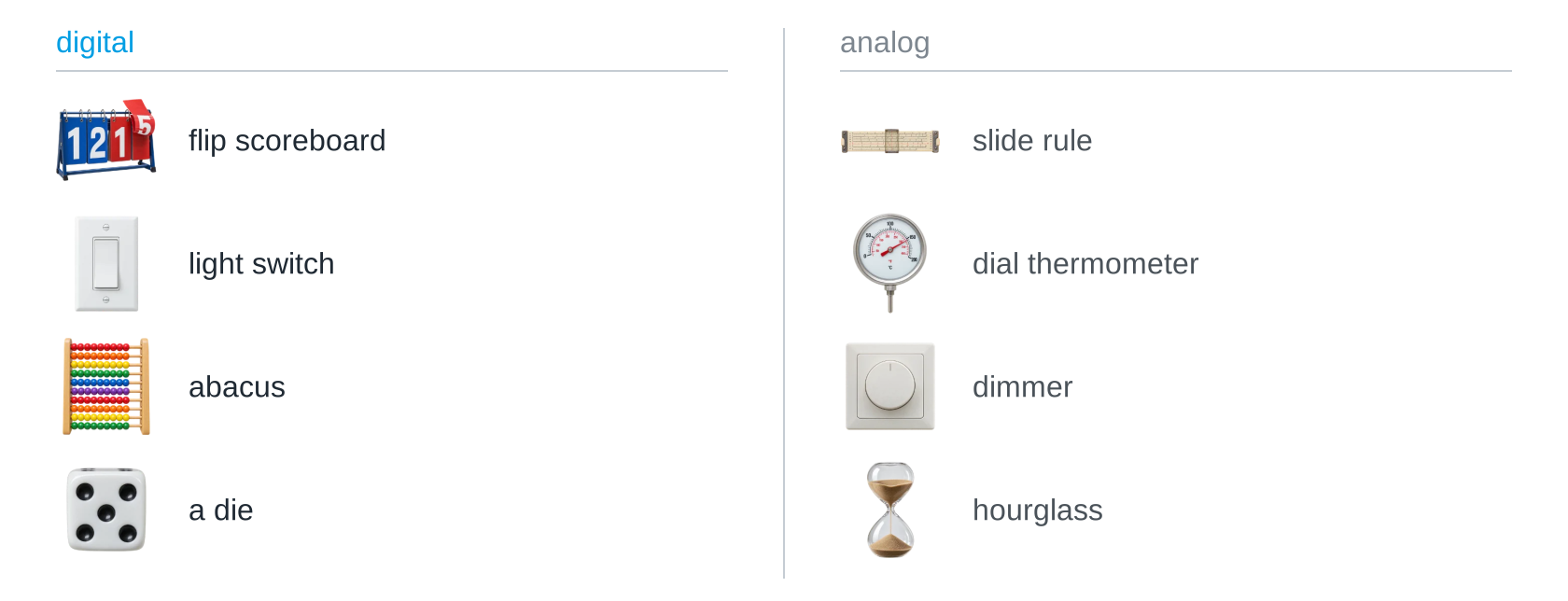
Figure 1: Not one of them contains a chip. Electronics is only today’s usual carrier, not the defining feature, and the reverse holds as well: an amplifier is electronic and still stepless.

So here is the definition, and it mentions no electricity at all: digital means finitely many states, and nothing in between counts. Both halves carry weight. The first is the harmless one. The second is where all the engineering hangs, because if nothing between the states counts, then nothing between the states can go wrong either.

The part no program controls

Your own link runs through all three zones. The sender turns numbers into light, the sensor turns light back into numbers: digital, analog, digital.

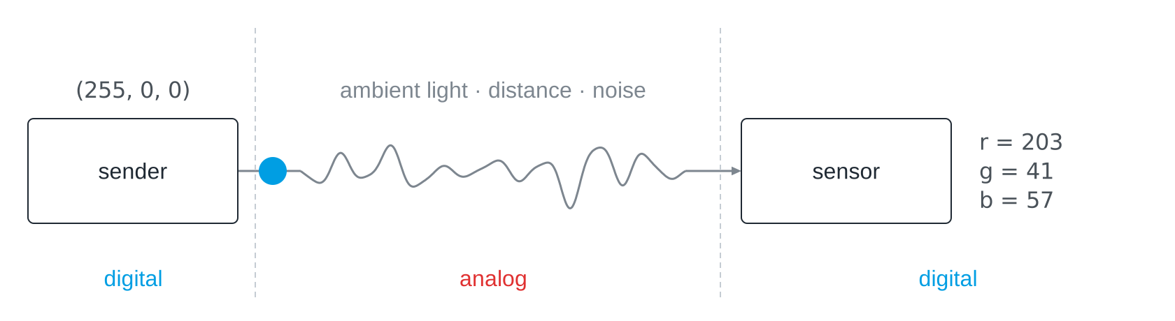
Figure 2: The middle is physics. It is stepless and disturbed by ambient light, distance and noise, and no program in the world controls it.

Light is analog: between any two brightnesses lies another, there is no smallest step. Your program needs the opposite, finitely many states that are clearly apart. Digitising a signal means nothing more than representing it by a finite sequence of numbers.

The margin, not the noise

How many states can you afford? That question has a picture, and it is the one to remember from this page.

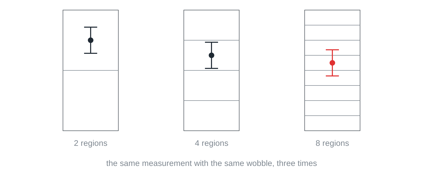
Figure 3: Three times the same measurement with the same wobble, and only the number of regions grows. With two regions the band sits comfortably inside its own region, with four it gets tight, with eight the same band crosses the boundary.

The noise did not grow. The margin shrank. The distance between regions is your safety reserve, and more regions spread the same reserve over more boundaries. The other half of that problem is on Signal und Rauschen: there the number of symbols stays put and the measuring gets faster instead. Both roads end at the same wall.

What the thrown-away precision buys

Digitising is a one-way street. Which of the infinitely many values inside a region it really was cannot be recovered afterwards. That is not an accident, it is the purchase price, and here is what you buy:

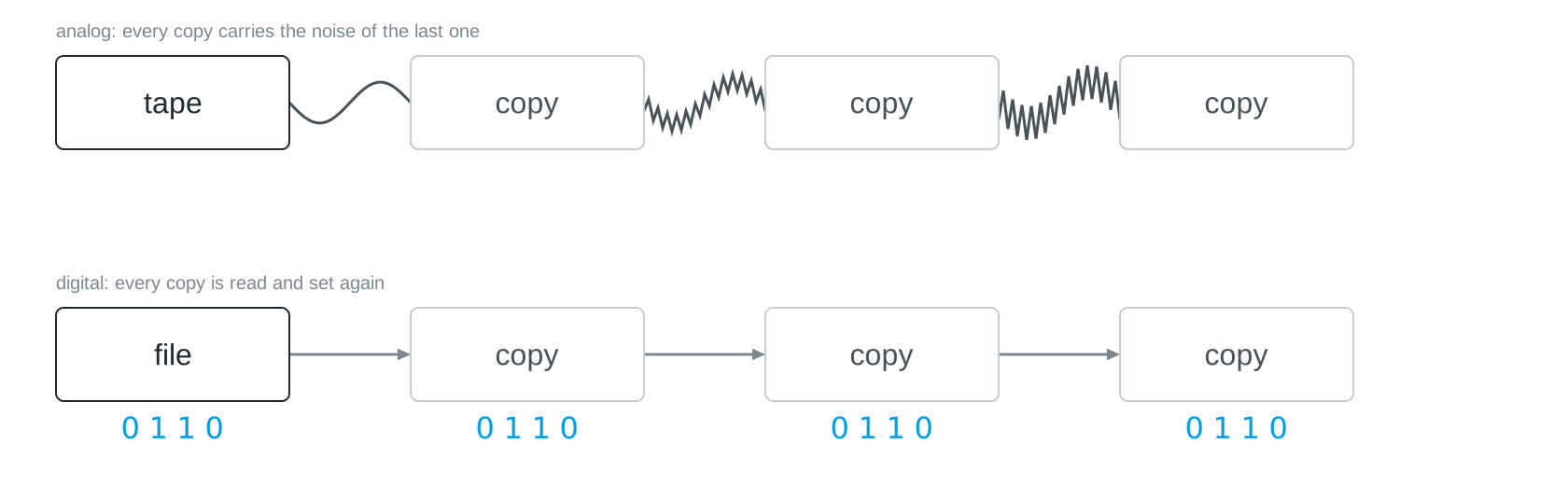
Figure 4: The tape copies its stepless wave along with all the noise and adds its own with every generation. The file is born again from clean states at every copy: read, set afresh, done.

Every disturbance smaller than the distance between states disappears completely in the process. That is why digital technology is reliable, not although it throws information away but because it does, and why the thousandth copy of a file is still the original. You can run that experiment yourself in The Copier: each press of “copy” hangs the next analog generation on the wall until the original has disappeared, and one button hangs the identical file copy next to it.

the copierpress copy and hang each generation on the wall: watch the analog picture fade copy by copy, then ask what a file would have done.LiFi Project · concept demos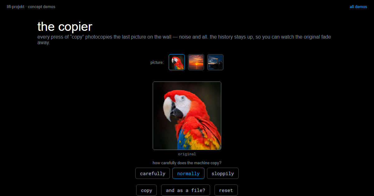

Two cuts

Digitising always takes two cuts, and a photo shows both of them.

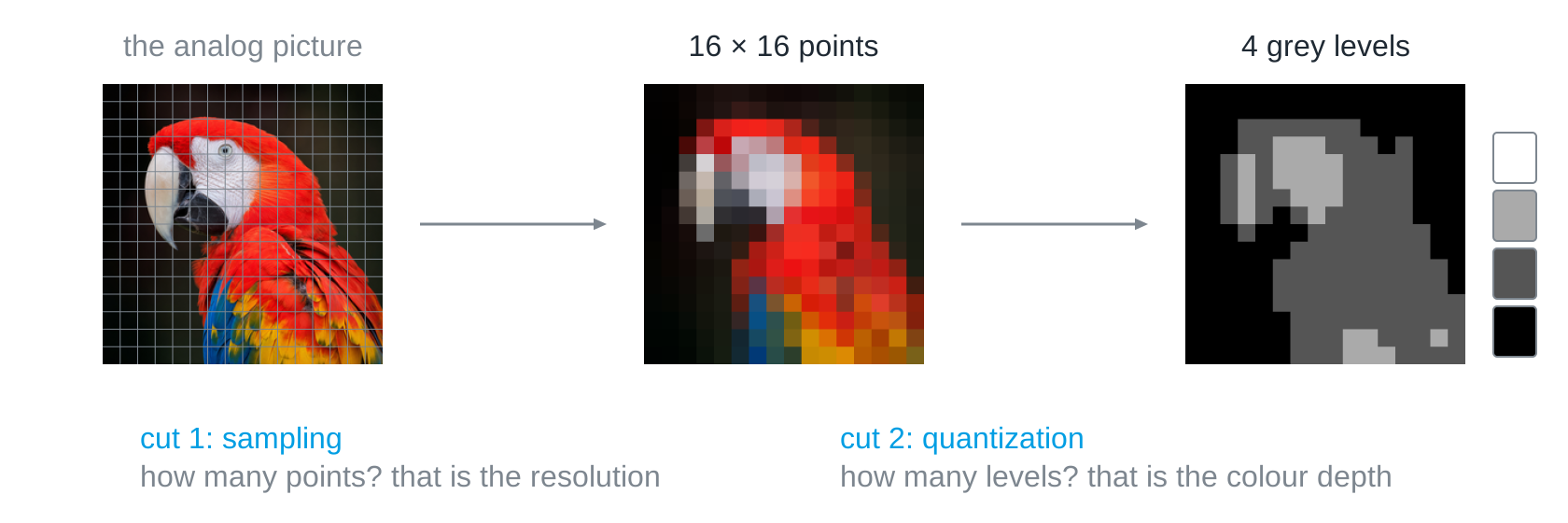
Figure 5: The first cut goes through the area, the second through the value.

The first cut turns the stepless picture into measuring points, sixteen by sixteen in the figure. That is sampling, and how fine it is is the resolution. The second cut rounds the brightness of every point to one of the agreed steps, four grey levels in the figure. That is quantization, and the number of steps is the colour depth. Those steps are exactly the regions from the section above, now applied to a picture.

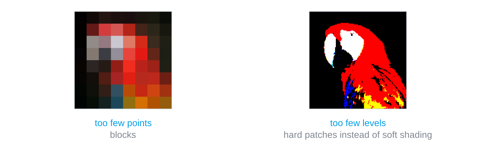
Both cuts leave different traces, and that is how you tell which knob to turn:

Figure 6: Blocks mean too few points. Hard patches in what should be soft shading mean too few levels.

What a picture costs

One piece of arithmetic carries every file size: points × bits per point.

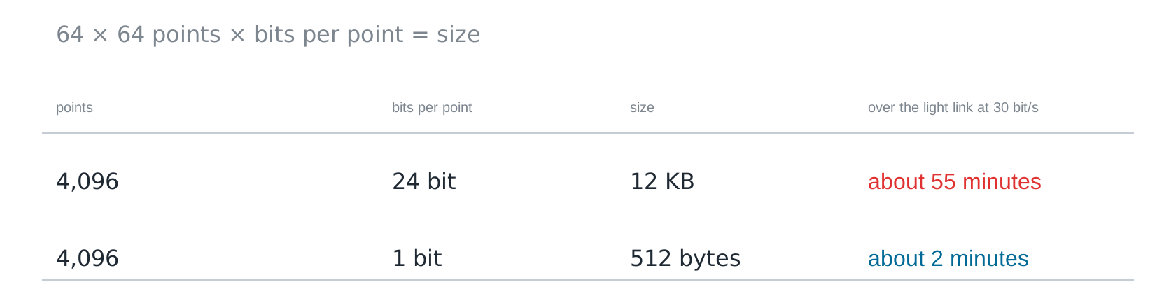
Figure 7: The same picture, one decision, fifty-three minutes of difference.

On your light link, size turns into time straight away. Which is why digitising is not a diligence exercise with “as fine as possible”, but a trade-off about which detail is worth the transmission time.

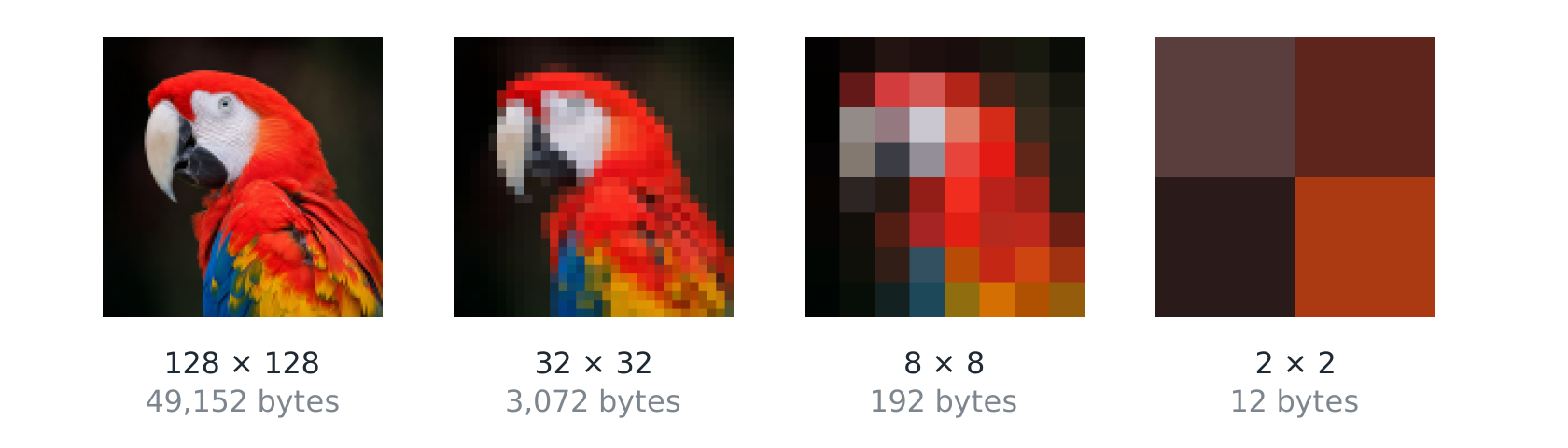
Figure 8: The same photo, ever coarser. Somewhere between the third and the fourth picture it stops being a parrot, and where exactly, people will disagree.

That disagreement is the point. There is no correct amount, there is only a trade-off, and in Challenge 4 you have 2 KB to make it in. You can play the whole thing through in The Photo Digitiser, from 256 by 256 points down to a single pixel, with colour depths from today’s standard through the sixteen colours of an early pc down to the four greys of the first Game Boy, and with the file size and the transmission time running along underneath.

the photo digitiserturn an analog photo into numbers: pick resolution and colour depth (down to the game boy's four greys), see the picture change, and watch the byte count grow.LiFi Project · concept demos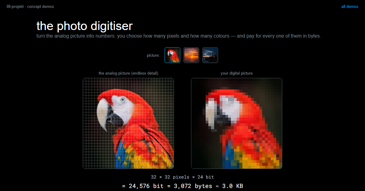

The same two cuts apply to sound. There, sampling slices time instead of area and the bit depth slices loudness instead of brightness; 44,100 samples per second at 16 bit is a CD. In The Audio Digitiser you can hear what each cut throws away.

the audio digitiserthe same two cuts for sound: choose sampling rate and bit depth, see the staircase on the wave — and hear what gets thrown away.LiFi Project · concept demos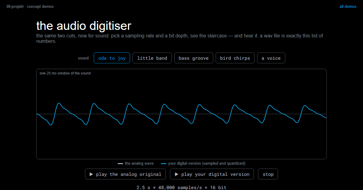

Where your own alphabet is born

At the end of all of this sits one line of your own code:

value = sensor.get_clear()

if value > 250:
    symbol = "bright"
else:
    symbol = "dark"

That threshold is the place where hundreds of possible readings turn into two symbols. It is not a constant of nature, it is your decision, and from there on it is your decision that holds, not the physics. Where it belongs does not come from your gut but from your measurement series: calibrate first, then compare (see Measuring and Experimenting).

Two colours are safe, eight are fast, and somewhere in between sits your alphabet. Only your own measurements know where, because the width of a region has to match the wobble of your readings.

Slides

The slides for this concept, right here. Page through them with the buttons in the top right corner, or click into the slides and use the arrow keys. The other buttons give you full screen, the slides in a new tab, and the deck as a PDF.

Practice questions

Try questions in the exam format here, with the answer and its reasoning shown right away.